Curve Ball and Newton Solvers

NOTE: This post assumes you are acquainted with first and second order optimisation techniques

Motivation

local-minima-meme Optimisation is probably the most important part for Deep learning. The main problems are the curse of dimensionality and irregular cost function topologies. Everything would have been so perfect if either one of these wouldn’t exist. SGD has become so popular, with the hope that, the stochastic noise added helps escaping the local optima and saddle points. But still this does’t work everytime.

Second order optimisers such as L-BFGS, CG and other quasi newton methods work very well in lower dimensions but they fail in the higher dimension because of the memory and computational growth is exponential w.r.t increase in dimension.

This paper proposes a new faster method - curve ball addressing the issues of 2nd order optimisers

Optimisation Methods

Let’s quickly review the standard optimisation problem and the methods to solve it

Optimisation Problem

A usual machine learning problem involves,
Finding an optimum $w^{*}$ which minimises(or max) the loss function $L(\phi(w))$, Objective may also be constrained. But we could add a penalty function and make it unconstrained, So let’s focus only on this
$$w^{*} = \underset{w}{\operatorname{argmin} L(\phi(w))} = \underset{w}{\operatorname{argmin} f(w)}$$

And $f(w)$ is defined as
$$f(w) = \sum_{i}L(\phi(w,x_{i}))$$

Here, $x_{i}$ is the input data point.
So, in short we need to find the global minima of the function $f$

Gradient Descent

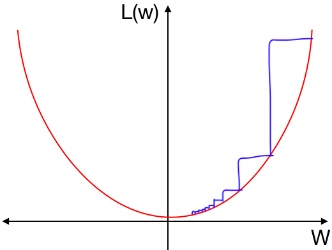GD-image I think this image best explains the Gradient Descent
The idea is to take the step in the direction of the gradient
The update rule for the iterate would be $$w_{t+1} = w_{t} - \alpha_{t}\nabla f(w_{t})$$

$\alpha_{t}$ is the learning rate or the step size at time t.
Note that this update rule is discretisation of the ode $$\dot{w} = -\nabla f(w)$$

$\nabla f(w) = \sum_{x_{i} \in dataset} \nabla_{w}L(\phi(w, x_{i}))$ It’s usually difficult to evaluate this term everytime (over all dataset).

So we approximate the term as
$$\nabla f(w) \approx \sum_{x_{i} \in batch} \nabla_{w}L(\phi(w, x_{i}))$$ and this gives us Stochastic Gradient Descent (actually mini-batch). Which is a noisy discretisation of above ode

\[\dot{w} = -\nabla f(w) + \xi\]

The convergence is noisy but it may or may not get stuck at local minima and saddle points

Newtons Method

This is actually a root finding method for a function f
Since, minima is the root of $\nabla f(w)$ we can use this update rule to findout the $$w_{t+1} = w_{t} - \frac{1}{\nabla^{2}f(w_{t})}\nabla f(w_{t})$$

We can think of this as newton’s method provides a value for the step size parameter $\alpha_{t}$ $$\alpha_{t} = \frac{1}{\nabla^{2}f(w_{t})}$$

For vector $\bar{w_{t}}$ we have, $$\bar{w_{t+1}} = \bar{w_{t}} - H^{-1}(w_{t})J(w_{t})$$

H, J are hessian and jacobian (of $f(w_{t})$) respectively

FMAD and RMAD

[WIP]